Something intuitive in the DAS (Data Availability Sampling) protocol is that if we increase the number of light nodes c, we can decrease the number of samples per light node s and vice versa. What is of interest is how the two numbers relate to each other while keeping the probability of block reconstruction the same. This is important when looking ahead to see if we can increase the square size by increasing the sample amount per light node if the network does not have enough light nodes yet.
This work is based on Fraud Proofs: Maximising Light Client Security and Scaling Blockchains with Dishonest Majorities and is meant for the Celestia community to help them make decisions about when to increase the square size.
Background
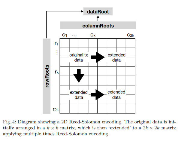
The original TX data gets erasure coded in 2 directions and gives the following diagram.
Theorem 4 from the Paper: The probability that the number of distinct elements sampled from a set of n elements, after c drawings with replacement of s distinct elements each, is at least all but λ elements:
Where W_i is defined as:
In the context of block reconstruction, it gives the following collary where the light nodes have to at least sample k(3k − 2) distinct shares from the 2k × 2k matrix in the worst case to guarantee the reconstruction of the full block:
Collary 1 from the paper: Given a 2k × 2k matrix E , where each of c players randomly samples s distinct shares from E. The probability that the players collectively sample at least γ = k(3k − 2) distinct shares is P_e(Z ≥ γ).
Results
Looking at the table in the paper, you start to see possible relationships between k, s, and c. If you double the number of samples, you can decrease the number of light nodes by 2. If you double the square size, you need four times as many light nodes.
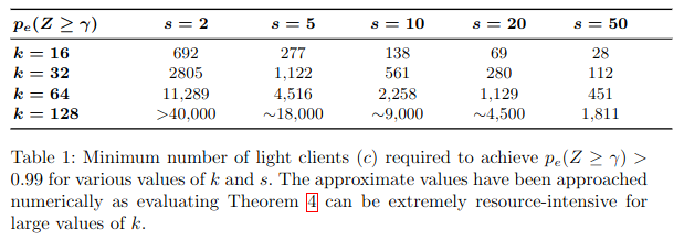
Relation ship between the number of light nodes c and the amount of samples s
From the table, we assume that the relationship between c and s is that if we double the light nodes c, we can half the number of samples s. We can generalize that to a factor of a.
We want to show that after altering the formula, the probability of block reconstruction stays the same.
Adjust c to c' = c/a and s to s' = sa. The modified W_i becomes:
The modified formula is:
What we have to show is that the probability stays the same.
If the last term of the sum is equal, then the rest of the sum is equal as well. Therefore we we only have to show that W_i^c = (W_i')^{c'}
Let`s substitute \lambda = 4k^2 - k(3k-2) and n = 4k^2 in W_i^c to get the following expression:
As we aim to increase the square size, we will have a large k, which means that we can apply stirling’s approximation \binom{n}{k} \approx \frac{n^k}{k!} for the binomial coefficients in W_i.
This will result in
We can aply the same steps to W_i' so the resulting (W_i')^{c'} will be the following:
From our original assumption that c' = c/a and s to s' = sa, these cancel each other out, and we conclude that (W_i ')^{c'} approximates (W_i)^{c}. This means that the block reconstruction probability will stay the same in large square sizes when we adjust the number of distinct samples and light nodes by a constant factor a.
Relationship between the square size k and the number of samples s
The original intuition is that the bigger the square size k, the more samples s you need for the same block reconstruction probability if the number of light nodes c is fixed. Looking at the table, when you double the square size and quadruple the number of samples, you can keep the same number of light nodes. This can be seen for the columns s=5 and s=20, where moving from k to 2k keeps the number of light nodes c roughly the same.
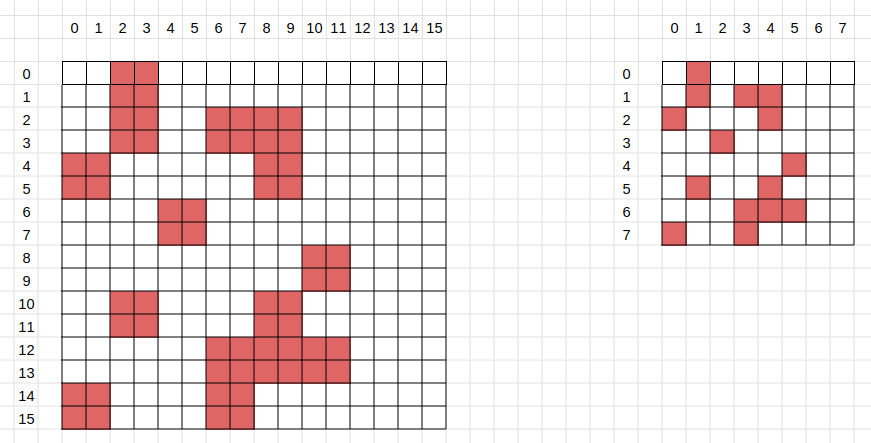
Here, we will explore the intuition more visually. Let’s assume we have a 2k × 2k matrix called E and need s samples per light node. Now, let’s project a 4k × 4k matrix E^* into E. This means that each share in E will now be a small 2 × 2 matrix consisting of 4 shares.
We needed s samples to sample E to get a certain block reconstruction probability. After the projection, each sample is now 4 samples in E*. Visually, you should see how this will keep the block reconstruction probability the same, as each row and column has the same individual block reconstruction probability.
The resulting intuition should be to not just increase the number of samples but also to group samples together if we want to save on the inclusion proof size of a sample. To apply this to the protocol a request for a sample could now receive a range of samples as a result instead of just one.
We must ensure that the probability of a light node detecting unavailable shares stays the same, so you can’t just request one sample and get a row of 16 shares. You still have to do 16 samples with an equal probability of hitting each quadrant, but the number of shares per sample can be increased without adding much bandwidth overhead.
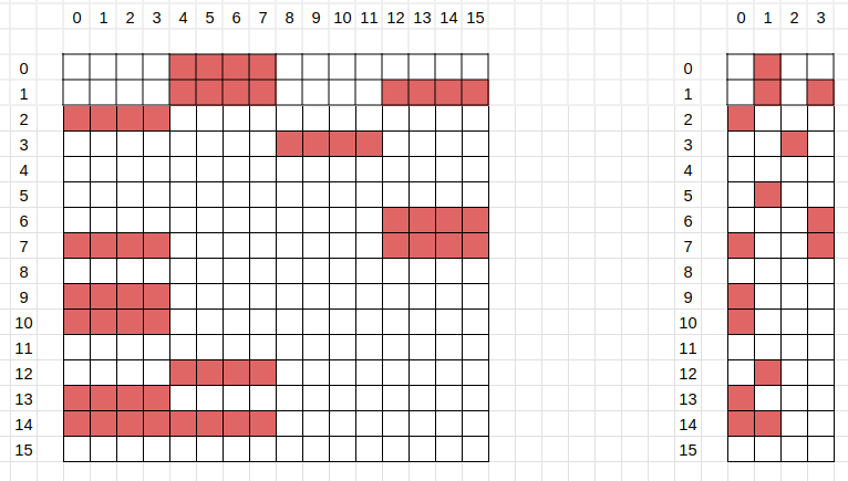
With the above projection, we would not get the full benefit of grouping shares to minimize inclusion-proof size. So, a different projection that could be explored is sampling, let’s say, four shares in a row. Let’s say that four shares in a row equal one share, which means that our projection would be from a 4k × 4k matrix to a k × 4k matrix.
The k × 4k matrix, the ODS would be 1/2k × 2 k matrix.
Let’s disregard the fact you can do reconstruction before the γ = k(3k − 2) worst-case scenario and stick to the papers lower bound. If we can reduce the number γ that is required, then we can increase the reconstruction probability if we keep s and c fixed. We can reduce the number γ by increasing the samples an attacker would have to withhold. Stretching the square into a rectangle using a projection has exactly this effect.
Surprisingly, sampling 16 samples 4 in a row gives you collectively better reconstruction probabilities than sampling 64 shares randomly in a quadrant. For that, we will compare different projections and how they affect γ.
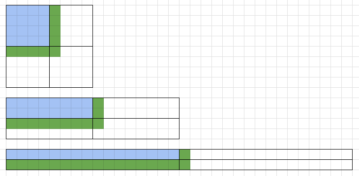
In the diagram below, you see a 2k × 2k matrix, a k × 4k matrix, and finally a 2 × (2k)^2 matrix. All of them erasure code the original square of k^2 in 2 dimensions, so the total area is n = 4k^2.
As per the paper, as an attacker, we not only have to withhold k * k data but also one extra share outside of the k * k square to prevent reconstruction using the erasure code.
We should look at the green shares as the blue ones stay the same. The flatter the rectangle, the more green shares the erasure coding will have. This will result in the attacker having to withhold more data in an attempted attack, which means that the flatter the rectangle, the smaller γ gets. This means c light clients — each sampling s distinct shares — must collectively sample less γ shares for the same reconstruction probability. Sampling the same number of shares gives you a better reconstruction probability in a flatter rectangle.
Therefore, we can conclude that making a projection where shares are grouped instead of distinct gives us at least the same or better reconstruction probability.
The conclusion is that to maintain the same reconstruction probability going from a square size of k to 2k, you must increase the number of samples s by 4 when keeping the number of light nodes fixed. As initially observed, this results in a quadratic relationship between s and k.
Conclusion:
- If you double the number of light nodes, you can halve the number of samples
- If you double the square size, you have to quadruple the number of samples
- You can save up on inclusion proof size when grouping shares together, so light nodes sampling more than 16 samples should sample in tuples or more instead of more distinct shares to save up on bandwidth.
This is the final simplified formula to calculate any given constellation with the assumptions of the paper:
\frac{c*s}{(2k)^2} \sim 1.37
c:= Amount of light nodes in the network
s:= Amount of samples per light node
k:= Square size of original data square
Acknowledgments
I want to thank @walldiss for our many productive discussions on this topic and feedback on this post.
