Context:
The faster the blocks go, the more load there will be on light nodes. Primarily, three things will see the load concerning storage and bandwidth on the side of the light node:
- Tendermint Header
- Commitment to the Erasure Coded Data(Currently the DAH)
- Sampling and Sample(+Proof) Size
Validators are constrained by:
- how fast/expensive it is to create the commitment to the erasure code
Full Nodes are constrained by:
- Amount of Light Nodes that can sample from it at the same time
- How hard it is to provide the Samples to the Light Node
If we decouple block finality from square creation and erasure coding, we must deliberately resource price against the abovementioned constraints.
Controlling the rate of square creations
An excellent way to keep the light node requirements in check is to control the square creation. This controls how often light nodes download the commitment and sample the erasure coding. If the square construction is too frequent, we have to decrease the rate of squares by making it more expensive to include transactions, including blob transactions. If the square takes too long to create, we can lower the gas fees to make it cheaper to include transactions, increasing the rate of squares.
Only after the square is created can light nodes sample for a data availability guarantee. The square construction is, therefore, blocking light node finality, so there should be a minimum light node finality that Celestia guarantees. A square can be created per block or span multiple blocks, forming one large square for a batch of blocks. Let’s call t_{square} the time it takes to create a square. There can be a maximum square time t_{square_{max}}, a minimum square time t_{square_{min}} and of course a target square time t_{square_{target}}.
t_{square_{min}} could be the block time, but it depends on how light nodes perform under fast block times. Issues might arise with syncing and validating headers and sampling. The same must be tested with full nodes to see if they can keep up syncing fast squares and handle this amount of samples.
t_{square_{max}} should not exceed the light node finality that Celestia guarantees. There could be a period of empty blocks, which could lead to the creation of the square at a frequency with bad UX for light nodes. Here, the bad UX would result from the time it takes for light nodes to get an availability guarantee, as this guarantee might block interactions with the light node. I think 30 seconds to 1 minute could be a good upper bound.
The t_{square_{target}} can be derived from the target consensus throughput the chain aims for.
Finally, we have to account for the fact that if we keep the number of samples constant, we cannot make the square arbitrarily large, as there could not be enough light nodes to make the reconstruction possible. This means if we want to achieve Level 4 security for our light nodes, we will have to cap the maximum square size. Therefore, the frequency of squares and the maximum square size is the upper bound of the throughput you can achieve with level 4 light nodes, assuming a fixed amount of samples per light node.
Observations on light node requirements
As shown in the introduction, light nodes have to download various things. Depending on how we construct the square, we can amortize different parts of the cost. Some things have a constant cost over the square, and some will scale linearly with the square’s size.
This section should explain whether or not we should wait for the square as long as possible.
Let’s assume that the validator set does not change in between squares. Therefore, a light node must validate one tendermint header in each square to ensure it follows consensus. This is a one-time cost and no matter how big the square is, the light node has to validate one thing, so it makes sense to wait as long as possible for the square.
Let’s look at the other 2 things light nodes have to download: the samples and the data availability header. In this construction, let’s assume that we have enough light nodes for level 4 light node security but cannot increase the square size; otherwise, there would not be enough samples to reliably reconstruct the square.
One solution is to quadruple the number of samples, with each square size doubling to keep the same reconstruction probability. That would mean that if squares come four times as slow and are four times as large, the light nodes would have to sample four times as much. This would defeat the purpose of delaying the square construction as a whole, as the same amount of data still has to be downloaded. For bigger squares, we are adding some overhead on a sample’s opening proof (inclusion proof) against the commitment (row/column root) that can be cleverly removed by combining samples in one proof—more on this in another post.
In relation to the square size, the Data Availability Header overhead lies in between. It consists of all the row and column roots. When the square size doubles, the size of the DAH doubles as we have twice the number of row roots and twice the number of column roots. This means that the DAH size scales proportional to the square root of the square’s area.
We could theoretically increase the square size to any size to decrease the light node requirements while maintaining the same throughput as the total amount needed for bandwidth and storage would decrease.
But it would be a burst download instead of distributing the load over time. A similar conclusion holds true for samples as well.
The overarching conclusion here is that it is not useful to think that just delaying the square as much as possible is the best solution. The function we are really trying to maximize here is the density of information inside the square, i.e., how much we can pack into the square. Therefore, if we control the rate of square construction, we need to ensure that it is tuned to maximize the density of useful information inside the square. Other options exist to reduce wasteful space apart from the square construction that can be tackled in parallel and will be explored in future posts.
Picking a suitable controller
The general idea is that light nodes can sustain a certain amount of bandwidth and storage requirements over a longer period. This means we are okay with having a burst of squares followed by less frequent squares when they average below our set node requirements.
To not reinvent this, we can pick a version of EIP-1559.
We can take several learnings from EIP-1559 to avoid the same mistakes. The first one is that there should be a sufficiently high minimum gas price; otherwise, there can be periods where the fee is close to nothing, making it not sustainable. Further reading can be seen in EIP-7762. The main reasoning behind the EIP is that price discovery of blobs was taking too long and they were basically free in Ethereum. We could use our current minimum gas price for this.
Another learning is to use an exponential EIP-1559 instead of a linear one. A good explanation with an example of the difference can be found by looking at how EIP-4844 changed the fee-market.
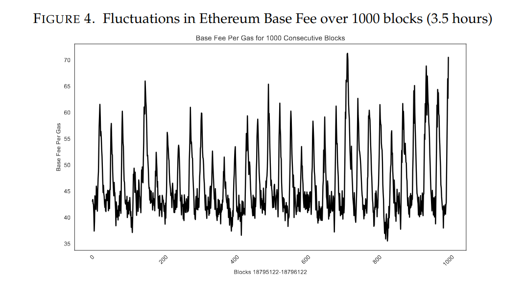
The latest learning is that the adjustment rate must be tuned; otherwise, we can see high fluctuations because of rapid updates from the controller. Users pay more than they should, but the gas target is achieved nonetheless. By differentiating the users as inpatient and patient regarding their inclusion, we get a TFM design more aligned with the real world. A great explainer showcases this and proposes one solution to adjust the rate change over time.
While adopting the EIP-1559 controller in the context of the rate of squares, the limit would be t_{square_{min}} (the fastest the squares could go) and the target t_{square_{targt}} ( derived from the target consensus throughput).
What are the next steps
First, we need a snapshot of sustainable light node requirements that we agree on. From these, we can extrapolate the rate and size of squares that are possible within the bounds of these requirements. Finally, we can tune a controller to ensure that the targeted requirements are met on average while not limiting the network’s burst usage. This will allow us to increase burst network throughput while having sustainable target throughput.
Shoutout
Thank you, @STB and @musalbas, for reading and reviewing this post.